This week, we will use the following packages as always, load them at the beginning of the session 👩 👨
library(tidyverse)
library(ggpubr)
library(DMwR) #dataset
#install.packages("package_name") #if you dont have one of them
Factors
Factors or the indicator variables and sets of indicator variables convert categorical predictors into numerical ones for regression models or plots. In R, each factor variable has levels, and those will take a real number from 1 to n number of factors in our variable; these numbers are determined alphabetically by default.
data("algae")
head(as_tibble(algae))
## # A tibble: 6 x 18
##   season size  speed  mxPH  mnO2    Cl   NO3   NH4  oPO4   PO4  Chla    a1    a2
##   <fct>  <fct> <fct> <dbl> <dbl> <dbl> <dbl> <dbl> <dbl> <dbl> <dbl> <dbl> <dbl>
## 1 winter small medi~  8      9.8  60.8  6.24 578   105   170    50     0     0
## 2 spring small medi~  8.35   8    57.8  1.29 370   429.  559.    1.3   1.4   7.6
## 3 autumn small medi~  8.1   11.4  40.0  5.33 347.  126.  187.   15.6   3.3  53.6
## 4 spring small medi~  8.07   4.8  77.4  2.30  98.2  61.2 139.    1.4   3.1  41
## 5 autumn small medi~  8.06   9    55.4 10.4  234.   58.2  97.6  10.5   9.2   2.9
## 6 winter small high   8.25  13.1  65.8  9.25 430    18.2  56.7  28.4  15.1  14.6
## # ... with 5 more variables: a3 <dbl>, a4 <dbl>, a5 <dbl>, a6 <dbl>, a7 <dbl>
Let’s look at the structure of the dataset.
str(algae[,1:8])
## 'data.frame':    200 obs. of  8 variables:
##  $ season: Factor w/ 4 levels "autumn","spring",..: 4 2 1 2 1 4 3 1 4 4 ...
##  $ size  : Factor w/ 3 levels "large","medium",..: 3 3 3 3 3 3 3 3 3 3 ...
##  $ speed : Factor w/ 3 levels "high","low","medium": 3 3 3 3 3 1 1 1 3 1 ...
##  $ mxPH  : num  8 8.35 8.1 8.07 8.06 8.25 8.15 8.05 8.7 7.93 ...
##  $ mnO2  : num  9.8 8 11.4 4.8 9 13.1 10.3 10.6 3.4 9.9 ...
##  $ Cl    : num  60.8 57.8 40 77.4 55.4 ...
##  $ NO3   : num  6.24 1.29 5.33 2.3 10.42 ...
##  $ NH4   : num  578 370 346.7 98.2 233.7 ...
As you can see, we got 3 categorical variables: Season, Size and Speed with different levels. To look at all the levels then you can use levels(df$variable).
levels(algae$size)
## [1] "large"  "medium" "small"
ANOVA
Analysis of variance is another type of linear model here, we will test that there is no difference in the mean \(\bar{y}\) of all the independent variable levels \(j\) also expressed as \(H_{0}: \bar{y}_j=0\). The F-statistic will compare the \(H_{0}\) with the \(H_{1}\) the alternative hypothesis. For the \(H_{1}\) at least one group with a mean function different from 0; \(H_{1}: \bar{y}_j\neq 0\). A larger value of F provides evidence against the \(H_{0}\) and in favor of the \(H_{1}\).
One-way ANOVA
Let’s use the function aov to calculate our One-way ANOVA.
fit_aov<-aov(mnO2~season,data=algae)
summary(fit_aov)
##              Df Sum Sq Mean Sq F value   Pr(>F)
## season        3  159.2   53.06   10.64 1.65e-06 ***
## Residuals   194  967.3    4.99
## ---
## Signif. codes:  0 '***' 0.001 '**' 0.01 '*' 0.05 '.' 0.1 ' ' 1
## 2 observations deleted due to missingness
Our F value is high, resulting in a significant difference \(P<0.05\). We can conclude that there is a difference in Manganese dioxide over seasons in our study area. However, we want to know the impact of each season on the area. As said before, ANOVA is also a linear model, so we will turn that ANOVA into a linear model with each season group being one factor.
summary.lm(fit_aov)
##
## Call:
## aov(formula = mnO2 ~ season, data = algae)
##
## Residuals:
##     Min      1Q  Median      3Q     Max
## -7.3798 -1.2148  0.4995  1.4972  4.5202
##
## Coefficients:
##              Estimate Std. Error t value Pr(>|t|)
## (Intercept)   10.6005     0.3531  30.025  < 2e-16 ***
## seasonspring  -2.5909     0.4696  -5.517 1.09e-07 ***
## seasonsummer  -1.1857     0.4878  -2.431 0.015980 *
## seasonwinter  -1.7207     0.4528  -3.800 0.000194 ***
## ---
## Signif. codes:  0 '***' 0.001 '**' 0.01 '*' 0.05 '.' 0.1 ' ' 1
##
## Residual standard error: 2.233 on 194 degrees of freedom
##   (2 observations deleted due to missingness)
## Multiple R-squared:  0.1413, Adjusted R-squared:  0.128
## F-statistic: 10.64 on 3 and 194 DF,  p-value: 1.649e-06
We can observe that the reference season is autumn and all the other seasons compared to this show a significant reduction (P<0.05). The biggest change is during spring, with a reduction of 2.59 mnO2 units. However, now we only have the differences compared to autumn; if we need a test for all the groups, we can use the Tukey’s range test.
Pairwise analysis
ANOVA will highlight any differences among the independent variable levels, but not which differences are significant. To establish each level as a treatment group and compare it with the rest in a post-hoc analysis, we will use TukeyHSD (Tukey’s Honestly-Significant Difference).
TukeyHSD(fit_aov)
##   Tukey multiple comparisons of means
##     95% family-wise confidence level
##
## Fit: aov(formula = mnO2 ~ season, data = algae)
##
## $season
##                     diff        lwr        upr     p adj
## spring-autumn -2.5908846 -3.8078479 -1.3739214 0.0000007
## summer-autumn -1.1857273 -2.4498770  0.0784225 0.0747333
## winter-autumn -1.7206613 -2.8941785 -0.5471441 0.0011041
## summer-spring  1.4051573  0.2198722  2.5904424 0.0128857
## winter-spring  0.8702233 -0.2178800  1.9583266 0.1658059
## winter-summer -0.5349340 -1.6755671  0.6056991 0.6178751
This output shows the pairwise differences between the seasons ($season).
- diff: difference in the mean between the \(n\) group and reference group \(j_{n}\)-\(j_{ref}\).
- lwr and upr: the lower and upper bounds of the 95% confidence interval.
- p-adj: the p-value of the difference.
After running pairwise comparisons among each group with a conservative error estimate, we found the groups that are statistically different from one another.
Look at the plot to understand the results better and observe those differences in the mean.
ggplot(algae,aes(x=season,y=mnO2,fill=season))+
  geom_point()+
  geom_boxplot()+
  theme_test()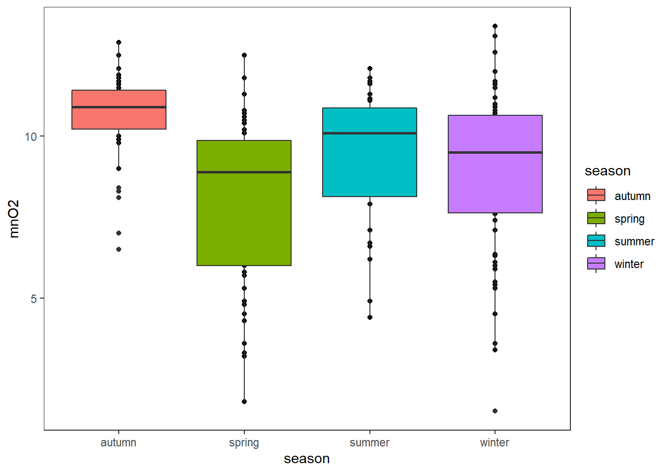
We can directly get some comparisons that perform one-sample Wilcoxon tests on vectors of data with the help of the package ggpubr.
ggplot(algae,aes(x=season,y=mnO2,fill=season))+
  geom_point()+
  geom_boxplot()+
  ggpubr::stat_compare_means(comparisons =list(c(1,2),c(1,3),c(1,4),c(2,3),c(2,4),c(3,4)),
                             label = "p.signif")+
  theme_test()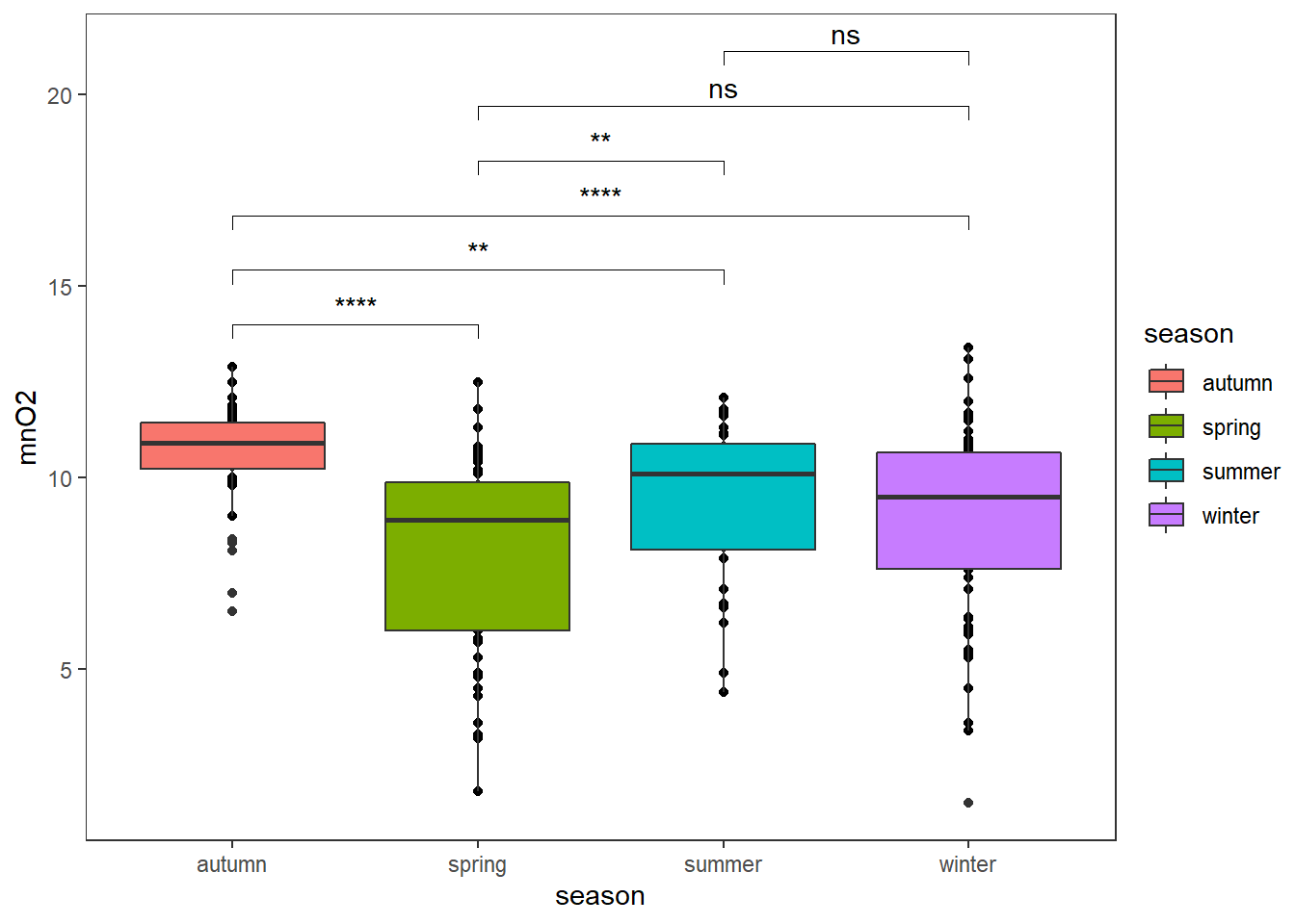
Two-way ANOVA
ANOVA type II follows the same ideas as our one-way ANOVA, testing the difference in the group means of our quantitative variable. Here, we will use two categorical independent variables. With the addition of this new variable, we will test how each independent variable affects the dependent variable as well as the interaction effect among them. Note that no significant interaction is assumed so we can continue with the analysis for main effects.
ggplot(algae,aes(x=season,y=mnO2,fill=size))+
  geom_violin()+
  theme_test()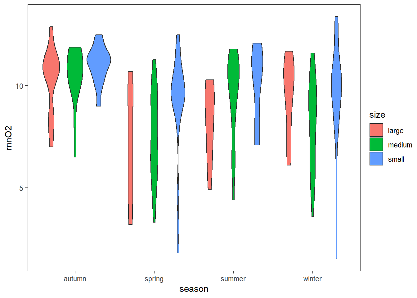
fit_aov<-aov(mnO2~season*size,data=algae)
summary(fit_aov)
##              Df Sum Sq Mean Sq F value   Pr(>F)
## season        3  159.2   53.06  11.086 9.94e-07 ***
## size          2   45.5   22.77   4.756  0.00967 **
## season:size   6   31.4    5.24   1.095  0.36703
## Residuals   186  890.3    4.79
## ---
## Signif. codes:  0 '***' 0.001 '**' 0.01 '*' 0.05 '.' 0.1 ' ' 1
## 2 observations deleted due to missingness
We get that season as expected rejects the \(H_o\) and so does size but there is no difference for different seasons and groups so we should remove the interaction term.
fit_aov<-aov(mnO2~season+size,data=algae)
summary(fit_aov)
##              Df Sum Sq Mean Sq F value   Pr(>F)
## season        3  159.2   53.06  11.053 9.99e-07 ***
## size          2   45.5   22.77   4.742  0.00977 **
## Residuals   192  921.7    4.80
## ---
## Signif. codes:  0 '***' 0.001 '**' 0.01 '*' 0.05 '.' 0.1 ' ' 1
## 2 observations deleted due to missingness
Post-hoc testing with Tukey’s Honestly-Significant-Difference (TukeyHSD) test lets us see which groups are different from one another.
TukeyHSD(fit_aov)
##   Tukey multiple comparisons of means
##     95% family-wise confidence level
##
## Fit: aov(formula = mnO2 ~ season + size, data = algae)
##
## $season
##                     diff        lwr         upr     p adj
## spring-autumn -2.5908846 -3.7851403 -1.39662888 0.0000004
## summer-autumn -1.1857273 -2.4262891  0.05483451 0.0667579
## winter-autumn -1.7206613 -2.8722816 -0.56904093 0.0008454
## summer-spring  1.4051573  0.2419887  2.56832601 0.0107692
## winter-spring  0.8702233 -0.1975769  1.93802352 0.1529061
## winter-summer -0.5349340 -1.6542838  0.58441581 0.6031445
##
## $size
##                     diff         lwr      upr     p adj
## medium-large 0.009204434 -0.94686616 0.965275 0.9997149
## small-large  1.009510198  0.01785058 2.001170 0.0449708
## small-medium 1.000305764  0.15944801 1.841164 0.0150440
This output shows the pairwise differences between the seasons ($season) and between the three levels of algae size ($size).
- diff: difference in the mean between the \(n\) group and reference group \(j_{n}\)-\(j_{ref}\).
- lwr and upr: the lower and upper bounds of the 95% confidence interval.
- p-adj: the p-value of the difference.
ANCOVA
Like ANOVA, “Analysis of Covariance” (ANCOVA) has a single continuous dependent variable. Unlike ANOVA, ANCOVA tests both a factor and a continuous independent variable (e.g., comparing carbon emission score by both ‘GDP’ and ‘continent’). The term for the continuous independent variable (IV) used in ANCOVA is named covariate. We will cover one-way ANCOVA and the classical model options.
Assumptions
ANCOVA makes several assumptions about the data, such as:
- Linearity between the covariate and the response variable for each level of the grouping variable. Test: Scatter plot of the covariate and the response variable.
- Homogeneity of regression slopes. The slopes of the regression lines, formed by the covariate and the outcome variable, should be the same for each group. This assumption evaluates that there is no interaction between the response and the covariate. The plotted regression lines by groups should be parallel.
- Normal Distribution, the response variable should be approximately normally distributed. Test:
Shapiro-Wilkof the model residuals. - Homoscedasticity or homogeneity of residuals variance for all groups. The residuals are assumed to have a constant variance. Test:
Levenefor the residuals and groups - No significant outliers in the groups. Test:
Model 4: Coincident Regressions for all levels
library(carData)#data set
fit_ancova<-aov(IQbio~IQfoster*class,data = Burt)
summary(fit_ancova)
##                Df Sum Sq Mean Sq F value   Pr(>F)
## IQfoster        1   5231    5231  83.382 9.28e-09 ***
## class           2    175      88   1.396    0.270
## IQfoster:class  2      1       0   0.007    0.993
## Residuals      21   1317      63
## ---
## Signif. codes: 0 '***' 0.001 '**' 0.01 '*' 0.05 '.' 0.1 ' ' 1- Non-significant interaction, so we should remove it.
- Categorical variable non-significant, so we may not need to consider it as there is no difference in the mean.
- Result is a linear regression.
fit_ancova<-aov(IQbio~IQfoster+class,data = Burt)
summary(fit_ancova)
##             Df Sum Sq Mean Sq F value  Pr(>F)
## IQfoster     1   5231    5231  91.259 1.8e-09 ***
## class        2    175      88   1.528   0.238
## Residuals   23   1318      57
## ---
## Signif. codes:  0 '***' 0.001 '**' 0.01 '*' 0.05 '.' 0.1 ' ' 1
summary.lm(fit_ancova) # same as summary(lm(IQbio~IQfoster+class,data = Burt))
...
## Coefficients:
## Estimate Std. Error t value Pr(>|t|)
## (Intercept) -0.6076 11.8551 -0.051 0.960
## IQfoster 0.9658 0.1069 9.031 5.05e-09 ***
## classlow 6.2264 3.9171 1.590 0.126
## classmedium 2.0353 4.5908 0.443 0.662
...A plot showing no effect of the categorical variable.
ggplot(Burt,aes(IQfoster,IQbio))+
  geom_point()+
  geom_smooth(method = "lm",se = T,colour="grey50")+
  geom_smooth(method = "lm",se=F,aes(colour=class))+
  labs(x="IQ-Child with foster parent",y="IQ-Child with biological parent")+
  theme_test()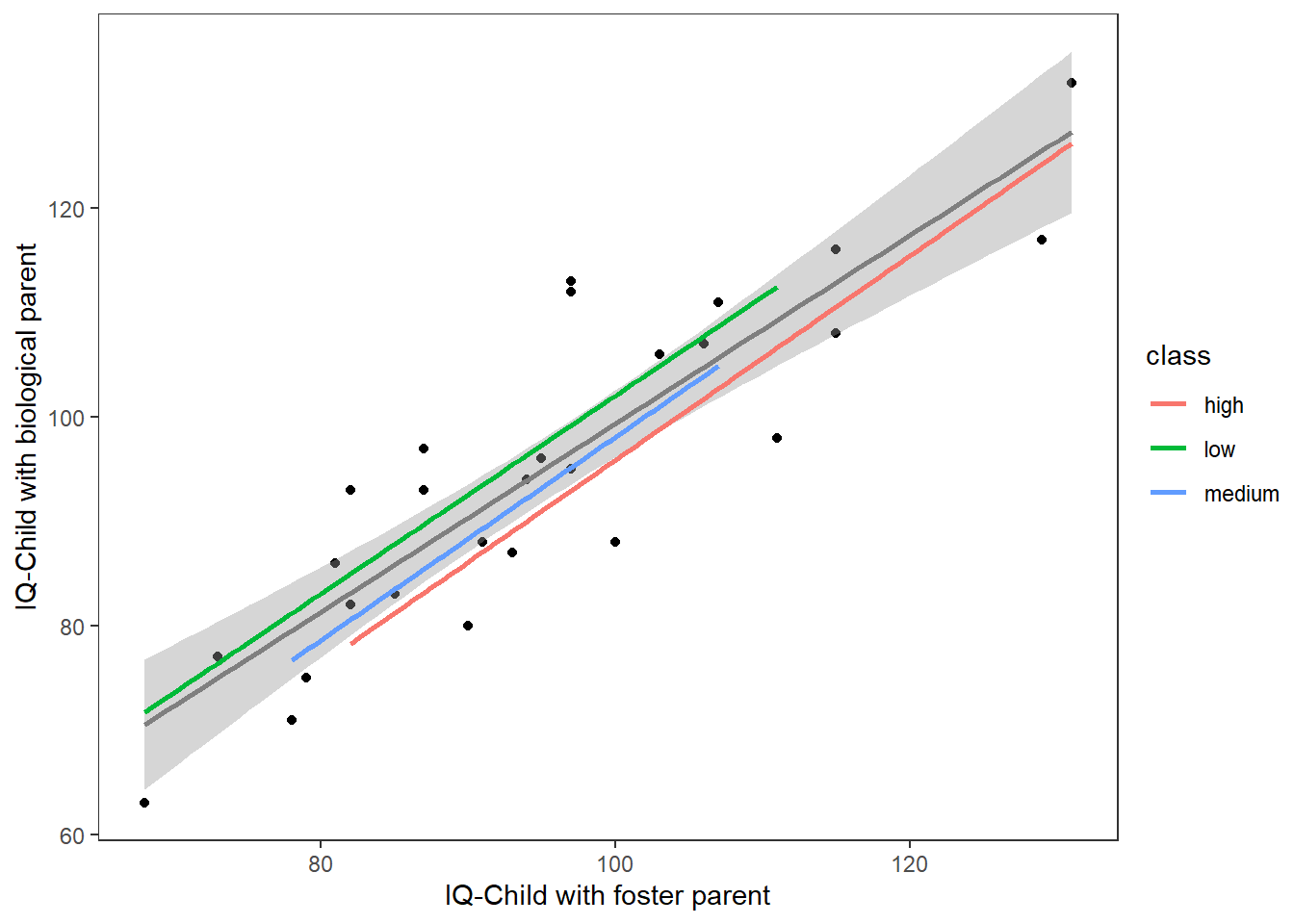
Model 3: Group Influence Regression Lines
Here, the levels of the categorical variable respond at different magnitudes with a change in the covariate. You may have the same intercept but, the critical indicator has different slopes and non-significant interaction.
fit_ancova<-aov(a3~Chla*season,data = algae[algae$a3!=0,])
summary(fit_ancova) #seasons significant
##              Df Sum Sq Mean Sq F value Pr(>F)
## Chla          1     68   67.81   1.222 0.2713
## season        3    931  310.18   5.588 0.0013 **
## Chla:season   3     18    5.86   0.105 0.9567
## Residuals   115   6384   55.51
## ---
## Signif. codes:  0 '***' 0.001 '**' 0.01 '*' 0.05 '.' 0.1 ' ' 1
## 3 observations deleted due to missingness
We tested the interaction assumption (interaction P>0.05), removing it from the ANCOVA.
fit_ancova<-aov(a3~Chla+season,data = algae[algae$a3!=0,])
summary(fit_ancova) #seasons significant
##              Df Sum Sq Mean Sq F value  Pr(>F)
## Chla          1     68   67.81   1.250 0.26581
## season        3    931  310.18   5.718 0.00109 **
## Residuals   118   6401   54.25
## ---
## Signif. codes:  0 '***' 0.001 '**' 0.01 '*' 0.05 '.' 0.1 ' ' 1
## 3 observations deleted due to missingness
Only seasons have an impact on algae species, and the ANCOVA analysis will look like the following.
ggplot(algae[algae$a3!=0,],aes(Chla,a3))+
  geom_point()+
  geom_smooth(aes(colour=season),method = "lm",se = F)+
  ggpubr::stat_regline_equation(aes(label =  paste(..eq.label.., ..rr.label.., sep = "~~~~"), color = season))+
  labs(x="Chlorophyll A",y="Algae species 3")+
  theme_test()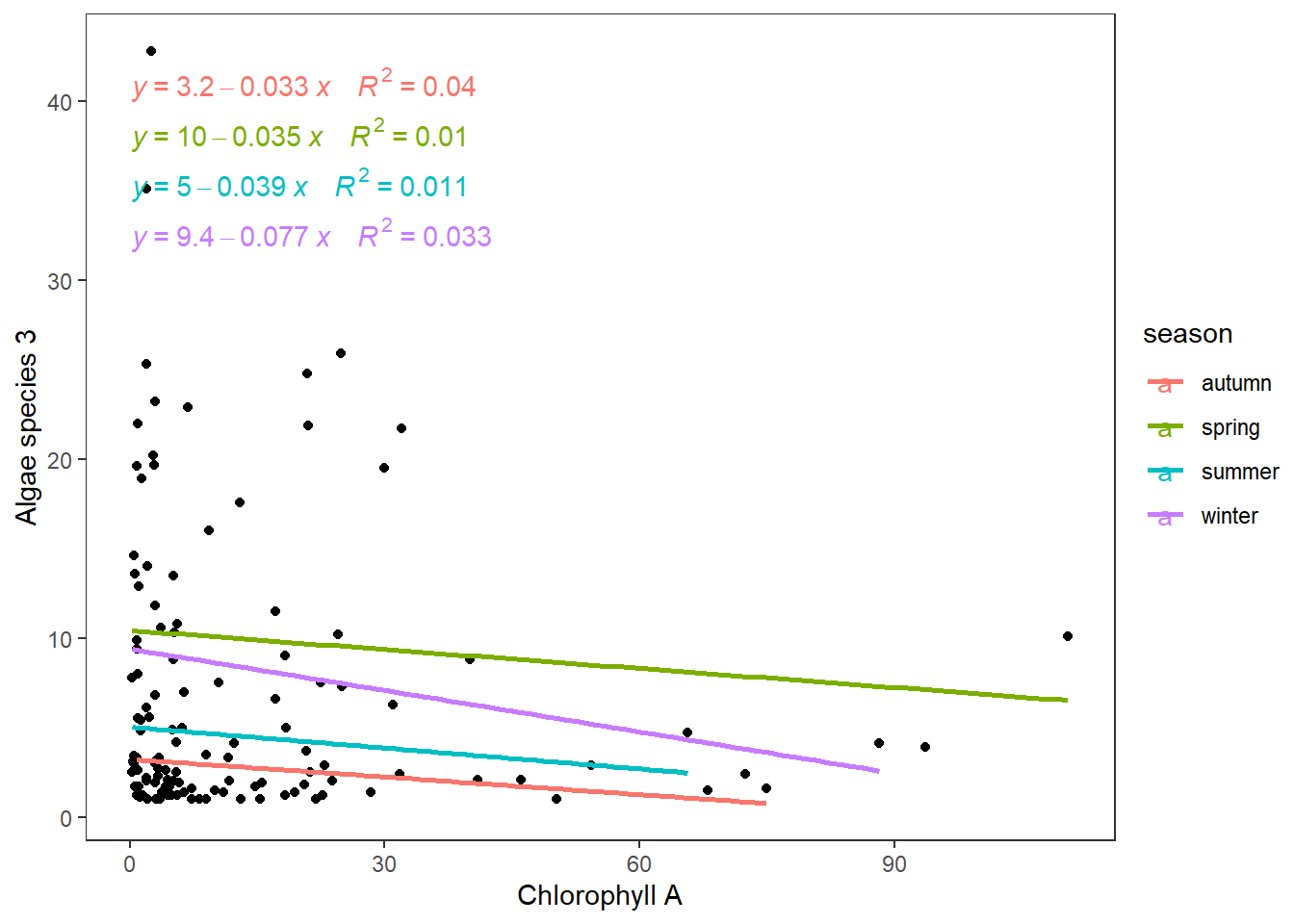
We can observe how lines change by different magnitudes (slopes \(\beta_j\)). During winter, the reduction is the biggest; however, they do not overlap with increasing values of Chlorophyll A.
Model 2: Parallel Regression Lines
For this model, there is a significant effect of classes/groups/levels, but this effect is identical (same slope) for all the groups as the continuous independent variable increases. This may be the perfect model for ANCOVA (highly unlikely to find it with random data).
x=seq(1,3,0.05)
df<-data.frame(x,
           y=c((1+.25*x),(2+.25*x),(3+.25*x)),
           group=c(rep("A",length(x)),rep("B",length(x)),rep("C",length(x))))
fit_ancova<-aov(y~x*group,data=df)
summary(fit_ancova)
##              Df Sum Sq Mean Sq   F value Pr(>F)
## x             1   2.69    2.69 4.828e+30 <2e-16 ***
## group         2  82.00   41.00 7.357e+31 <2e-16 ***
## x:group       2   0.00    0.00 1.520e+00  0.223
## Residuals   117   0.00    0.00
## ---
## Signif. codes:  0 '***' 0.001 '**' 0.01 '*' 0.05 '.' 0.1 ' ' 1
As expected there is no interaction between the categorical variable and covariate. The plot of this model would look something like this:
ggplot(data=df,aes(x=x,y=y))+
  geom_point()+
  geom_smooth(aes(colour=group),method = "lm",se = F)+
  ggpubr::stat_regline_equation(aes(label =  paste(..eq.label.., ..rr.label.., sep = "~~~~"), color = group))+
  scale_y_continuous(limits = c(0,5))+
  theme_test()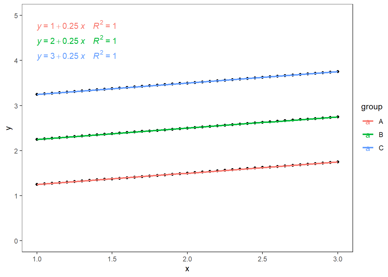
Model 1: Unrelated Regression Lines
This is the model more familiar to us. In this case, our regressions crossover, yet there is no significant interaction between the covariate and categorical variables. This is required for ANCOVA if you encounter a significant interaction, you can use moderated regression, which allows the interaction. The effect of the covariate is different for each level of our group.
df<-filter(algae,a3!=0,a3<20,mxPH>7)
fit_ancova<-aov(a3~mxPH*season,data=df)
summary(fit_ancova)
##              Df Sum Sq Mean Sq F value  Pr(>F)
## mxPH          1    5.0    4.95   0.237 0.62747
## season        3  289.4   96.46   4.613 0.00451 **
## mxPH:season   3   46.2   15.39   0.736 0.53290
## Residuals   105 2195.7   20.91
## ---
## Signif. codes:  0 '***' 0.001 '**' 0.01 '*' 0.05 '.' 0.1 ' ' 1
The plot would look like this:
ggplot(filter(algae,a3!=0,a3<30,mxPH>7),aes(mxPH,a3))+
  geom_point()+
  geom_smooth(aes(colour=season),method = "lm",se = F)+
  ggpubr::stat_regline_equation(aes(label =  paste(..eq.label.., ..rr.label.., sep = "~~~~"), color = season),
                                label.x.npc = .59)+
  labs(x="Chlorophyll A",y="Algae species 3")+
  theme_test()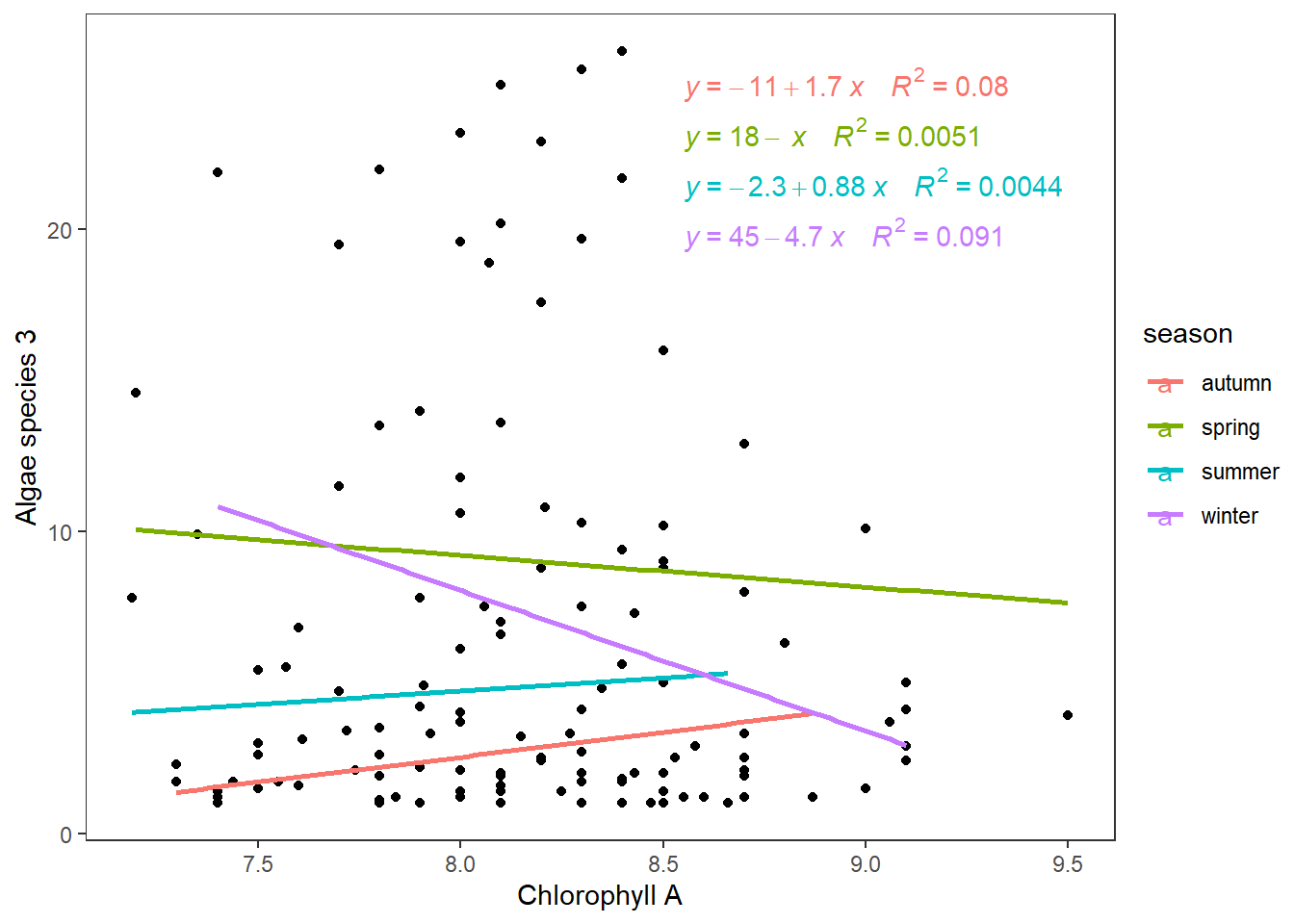
The models we used did not test the assumptions, and some may not be satisfied. Therefore, when doing your analysis, make sure you follow the steps highlighted in this and previous posts.