👩 This week, we will use the following packages as always, load them at the beginning of the session 👨.
library(tidyverse)
library(EnvStats)
We will cover the steps you will need when the assumptions of linear regression are not met. If you remember the assumptions for regression are the following:
- Normality
- Linearity \(E(Y|X)=F(x)\)
- Homoscedasticity \(Var(Y|X)=\sigma^2\)
We should ensure that the model fitted meets all the assumptions. But what if it does not ???
Usually, having a constant variance over the range of prediction (Homoscedasticity) is a bit problematic. If there is non-constant variance, you will need to give weights to the cases to match the variances among your points.
Larger weights causes smaller variance \(Var(y_{i}|Xi)=\sigma^2/w_{i}\) where \(i=1,...n\) and weights \(w_{i}>0\) are known levels. Let’s take the sleeping time of animals as an example.
data(msleep)
ggplot(msleep,aes(x=bodywt,y=sleep_total))+
  geom_point()+
  theme_bw()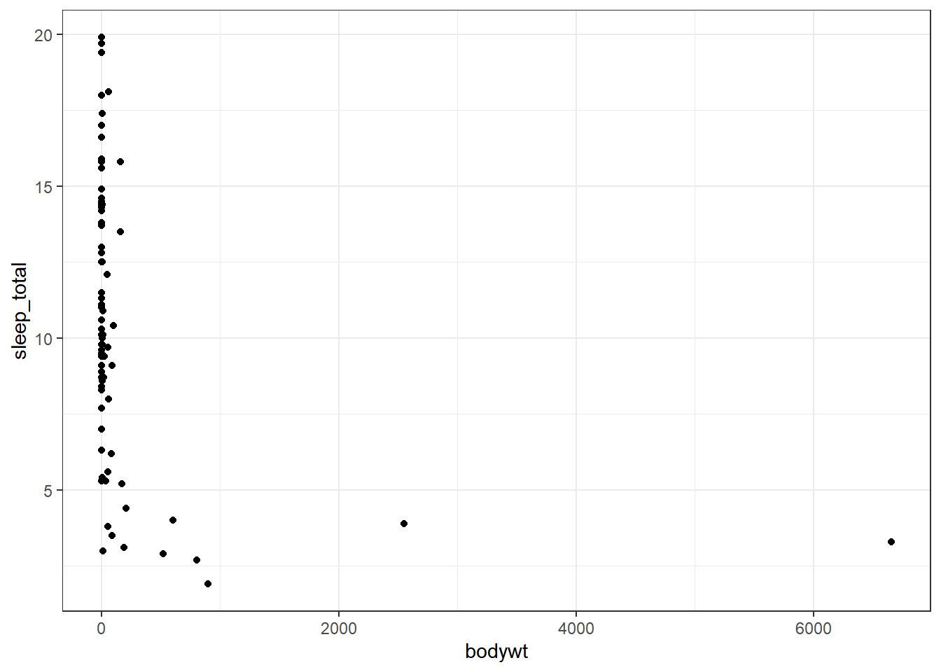
Clearly, we do not have a normal distribution; some animals have considerable bodyweight. We will use a log transformation to have a better distribution.
msleep$bodywt<-log(msleep$bodywt)
msleep$bodywt[16]
## [1] 0
msleep$bodywt[16]<-0.0000001
Now body weight is more uniform with a distribution closer to normal. Notice that with log-transformation, we encounter a species with a bw=0, so we changed that value as little as possible for our regression analysis because you will get an error if you use 0.
fit_lm<-lm(sleep_total~bodywt,msleep)
summary(fit_lm)
##
## Call:
## lm(formula = sleep_total ~ bodywt, data = msleep)
##
## Residuals:
##     Min      1Q  Median      3Q     Max
## -6.4991 -2.5671 -0.1683  2.0471 10.1928
##
## Coefficients:
##             Estimate Std. Error t value Pr(>|t|)
## (Intercept)  11.0891     0.4178  26.542  < 2e-16 ***
## bodywt       -0.7771     0.1249  -6.222 2.05e-08 ***
## ---
## Signif. codes:  0 '***' 0.001 '**' 0.01 '*' 0.05 '.' 0.1 ' ' 1
##
## Residual standard error: 3.683 on 81 degrees of freedom
## Multiple R-squared:  0.3233, Adjusted R-squared:  0.315
## F-statistic: 38.71 on 1 and 81 DF,  p-value: 2.046e-08
Now to add weights into the model, you will need the parameter weights and type a formula that will be added to each \(x_i\)
fit_weights<-lm(sleep_total~bodywt,weights = (1/msleep$bodywt^2),data=msleep)
summary(fit_weights)
##
## Call:
## lm(formula = sleep_total ~ bodywt, data = msleep, weights = (1/msleep$bodywt^2))
##
## Weighted Residuals:
##    Min     1Q Median     3Q    Max
## -2.044  0.075  1.397  2.926 97.917
##
## Coefficients:
##               Estimate Std. Error    t value Pr(>|t|)
## (Intercept)  8.300e+00  1.490e-06  5.571e+06   <2e-16 ***
## bodywt      -1.625e+00  1.635e+00 -9.940e-01    0.323
## ---
## Signif. codes:  0 '***' 0.001 '**' 0.01 '*' 0.05 '.' 0.1 ' ' 1
##
## Residual standard error: 14.81 on 81 degrees of freedom
## Multiple R-squared:  0.01204,    Adjusted R-squared:  -0.0001536
## F-statistic: 0.9874 on 1 and 81 DF,  p-value: 0.3233
Our two models will look like the following:
ggplot(msleep,aes(x=bodywt,y=sleep_total))+
  geom_point()+
  geom_line(data=fortify(fit_lm),aes(x=bodywt,y=.fitted),colour="blue")+
  geom_line(data=fortify(fit_weights),aes(x=bodywt,y=.fitted),colour="red")+
  annotate("text",x=c(3,6.5),y=c(-1,9),
           label=c(expression("W== 1/x[i]^2"),
                   expression("lm~model")),parse=T, #must be included to have the right format
           colour=c("red","navy"), #different colours for each text
           size=8)+
  theme_test()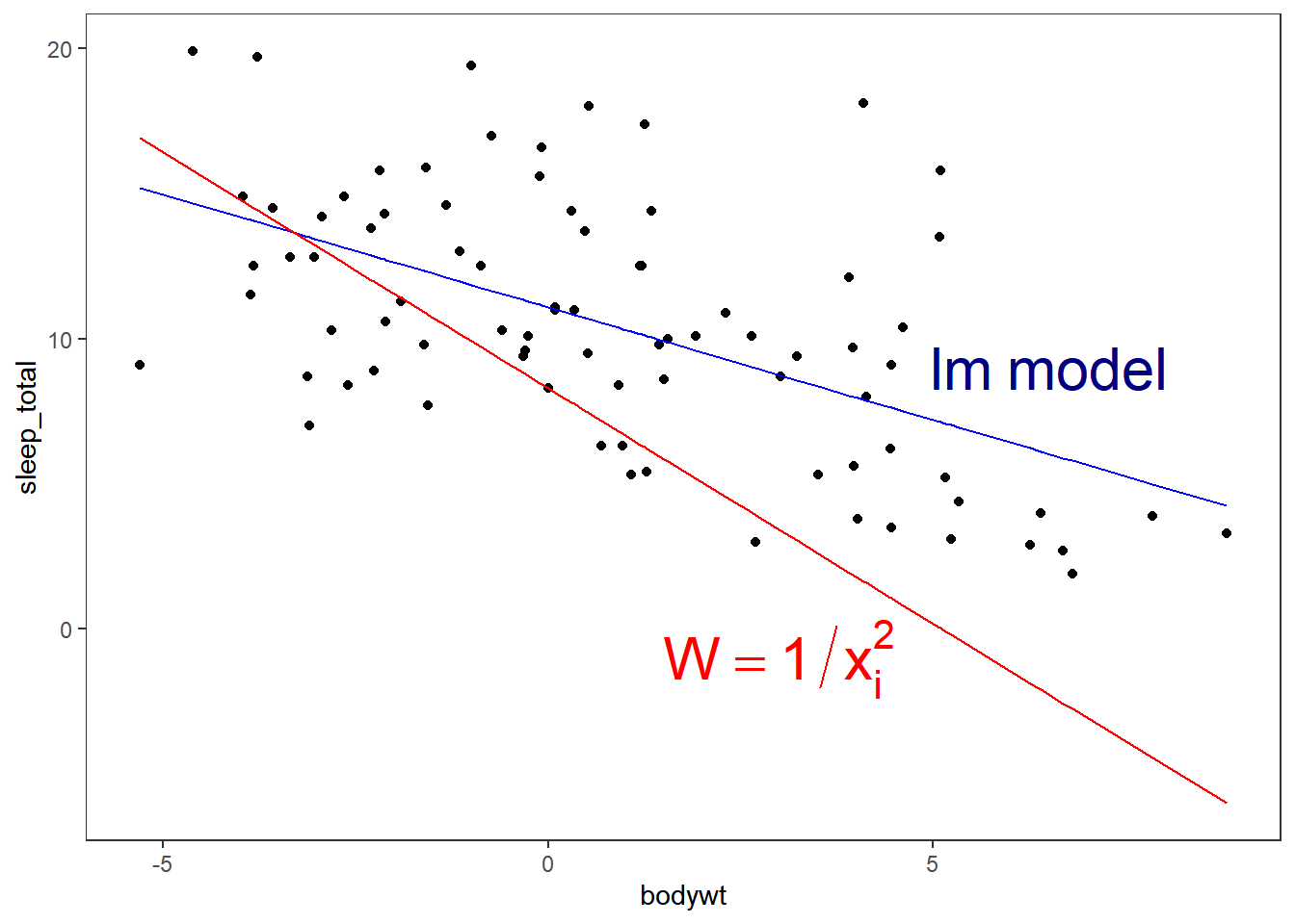
Lack-of-Fit Methods
This part will cover some model checking methods to decide if the mean function used to obtain a fitted model is reasonable in a particular regression. That is, whether there is something wrong with the observations for which the fit is not good.
Visual Lack-of-Fit with Smooths
ggplot(msleep,aes(x=bodywt,y=sleep_total))+
  geom_point()+
  geom_smooth(aes(outfit=regressionvalues_02<<-..y..),span=0.2,colour="steelblue",se=F)+
  geom_smooth(aes(outfit=regressionvalues_05<<-..y..),span=0.5,colour="darkgreen",se=F)+
  geom_smooth(aes(outfit=regressionvalues_09<<-..y..),span=0.9,colour="violet",se=F)+
  geom_smooth(aes(outfit=regressionvalues_00<<-..y..),colour="orange",se=F)+
  stat_smooth(method = "lm",colour="tomato",se=F)+
  annotate("text",x=7,y=c(19.5,18,17,16,15),label=c(bquote("Smoothness value="~alpha),"0.2","0.5","0.9","default") ,colour=c("black","steelblue","darkgreen","violet","orange"),parse=T)+
  theme_test(base_size=16)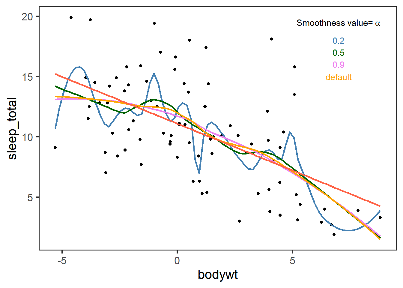
Ggplot with geom_smooth or stat_smooth use by default a smooth polynomial regression. That is, for the fit at point \(x\), the fit is made using points in a neighborhood of \(x\), weighted by their distance from \(x\) (with differences in ‘parametric’ variables being ignored when computing the distance). The size of the neighborhood is controlled by \(\alpha\) (set by span=x as in the previous plot). You can find more information here.
We added outfit to the geom_smooth in order to store the ..y.. values of the fitted regression in a new variable<-. It will only give you 80 points.
head(regressionvalues_00,20)
##  [1] 13.35127 13.33551 13.31757 13.29744 13.27509 13.25049 13.22363 13.19449
##  [9] 13.16304 13.12927 13.09314 13.05464 13.01375 12.97037 12.92343 12.87250
## [17] 12.81739 12.75796 12.69405 12.62550
In these course we focus in linear model but geom_smooth can integrate all types of
models=(e.g. “lm”, “glm”, “gam”, “loess” or a function from other packages MASS::rlm or mgcv::gam) andformulas=(e.g. y ~ x, y ~ poly(x, 2), y ~ log(x)) once specified.
Lack-of-Fit Based on Variance
We will test if our model has too much variation due to a lack of fit with an F-test. Let’s bring our initial lm and get the ANOVA results.
anova(fit_lm)
## Analysis of Variance Table
##
## Response: sleep_total
##           Df  Sum Sq Mean Sq F value    Pr(>F)
## bodywt     1  525.14  525.14  38.707 2.046e-08 ***
## Residuals 81 1098.93   13.57
## ---
## Signif. codes:  0 '***' 0.001 '**' 0.01 '*' 0.05 '.' 0.1 ' ' 1
The RSS are 1098.925779. We will break the Residual Sum of Squares into SSLF:Sum of Squares Lack of Fit and SSPE: Sum of Squares pure error.
olsrr::ols_pure_error_anova(fit_lm)
##    Lack of Fit F Test
## ------------------------
## Response :   sleep_total
## Predictor:   bodywt
##
##                        Analysis of Variance Table
## ------------------------------------------------------------------------
##                 DF     Sum Sq     Mean Sq      F Value        Pr(>F)
## ------------------------------------------------------------------------
## bodywt           1    525.1398    525.1398    105027.95    7.307278e-128
## Residual        81    1098.926    13.56698
##  Lack of fit    80    1098.921    13.73651     2747.302        0.0151741
##  Pure Error      1       0.005       0.005
## ------------------------------------------------------------------------
EnvStats::anovaPE(fit_lm)
##                   Df  Sum Sq Mean Sq  F value   Pr(>F)
## bodywt             1  525.14  525.14 105028.0 0.001964 **
## Lack of Fit       80 1098.92   13.74   2747.3 0.015174 *
## Pure Error         1    0.01    0.01
## ---
## Signif. codes:  0 '***' 0.001 '**' 0.01 '*' 0.05 '.' 0.1 ' ' 1
The F-statistic \(F^*=\frac{MSLF}{MSPE}\) for the Lack of fit helps us in testing:
- \(H_0\): The relationship assumed in the model is reasonable, i.e., there is no lack of fit \(\mu_i=\beta_0+\beta_1X_i\).
- \(H_A\): The relationship assumed in the model is not reasonable, i.e., there is lack of fit \(\mu_i\neq\beta_0+\beta_1X_i\).
In our example, the P-value is small than the significance level α, meaning that we reject the null hypothesis \(H_0\) in favor of the alternative \(H_A\). Therefore, there is enough evidence at the α level to conclude a lack of fit in the current model.
We get similar lack of fit results with the weighted regression:
olsrr::ols_pure_error_anova(fit_weights)
##    Lack of Fit F Test
## ------------------------
## Response :   sleep_total
## Predictor:   bodywt
##
##                         Analysis of Variance Table
## --------------------------------------------------------------------------
##                 DF     Sum Sq       Mean Sq       F Value        Pr(>F)
## --------------------------------------------------------------------------
## bodywt           1    216.5156        216.5156    43303.12    2.68224e-112
## Residual        81       1e+28    1.234568e+26
##  Lack of fit    80       1e+28        1.25e+26     2.5e+28     5.03052e-15
##  Pure Error      1       0.005           0.005
## --------------------------------------------------------------------------
Therefore, we should add better weights; if not, we can test our models.
Model comparison
Now we can find out which model is the best fit for our data using Akaike information criterion (AIC) model selection and aictab from the AICcmodavg package.
AIC calculates the best-fit model by finding the model that explains the largest amount of variation in the response variable while using the fewest parameters.
library(AICcmodavg)
aictab(list(fit_lm,fit_weights),modnames = c("Normal LM","Weighted LM"))
##
## Model selection based on AICc:
##
##             K   AICc Delta_AICc AICcWt Cum.Wt      LL
## Normal LM   3 456.26       0.00      1      1 -224.98
## Weighted LM 3 754.31     298.05      0      1 -374.00
The model that fits our data the best will be at the top. In this example, our Normal LM.