This week we will use the following packages as always, load them at the beginning of the session👨👩
library(tidyverse)
library(car)
library(dae) #install.packages("dae")
library(car)
library(DMwR)
library(olsrr)
library(plotly)
#install.packages("package_name")
Linear regressions can fit any data; this also means that you may get similar regression results even with different data because you fit the best option to reduce the variance between your points. Let`s look at the following plots with similar regression results,\(\sigma^2\), and \(R^2\) but with different observations and distributions.
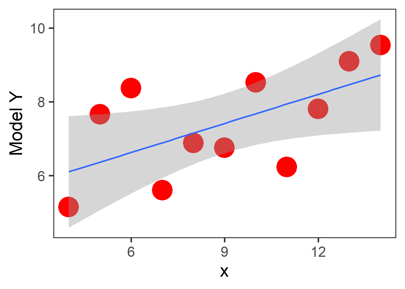
Some of these plots may be extreme cases, and it does not require statistical analysis to determine that one point is influencing our regression, but in the case of outliers, it may not be that obvious. Therefore, for general practice as mention in assumptions for linear regression it is required that you look at the residual plots.
fit.1<-lm(Model~x,plots)
residualPlot(fit.1)
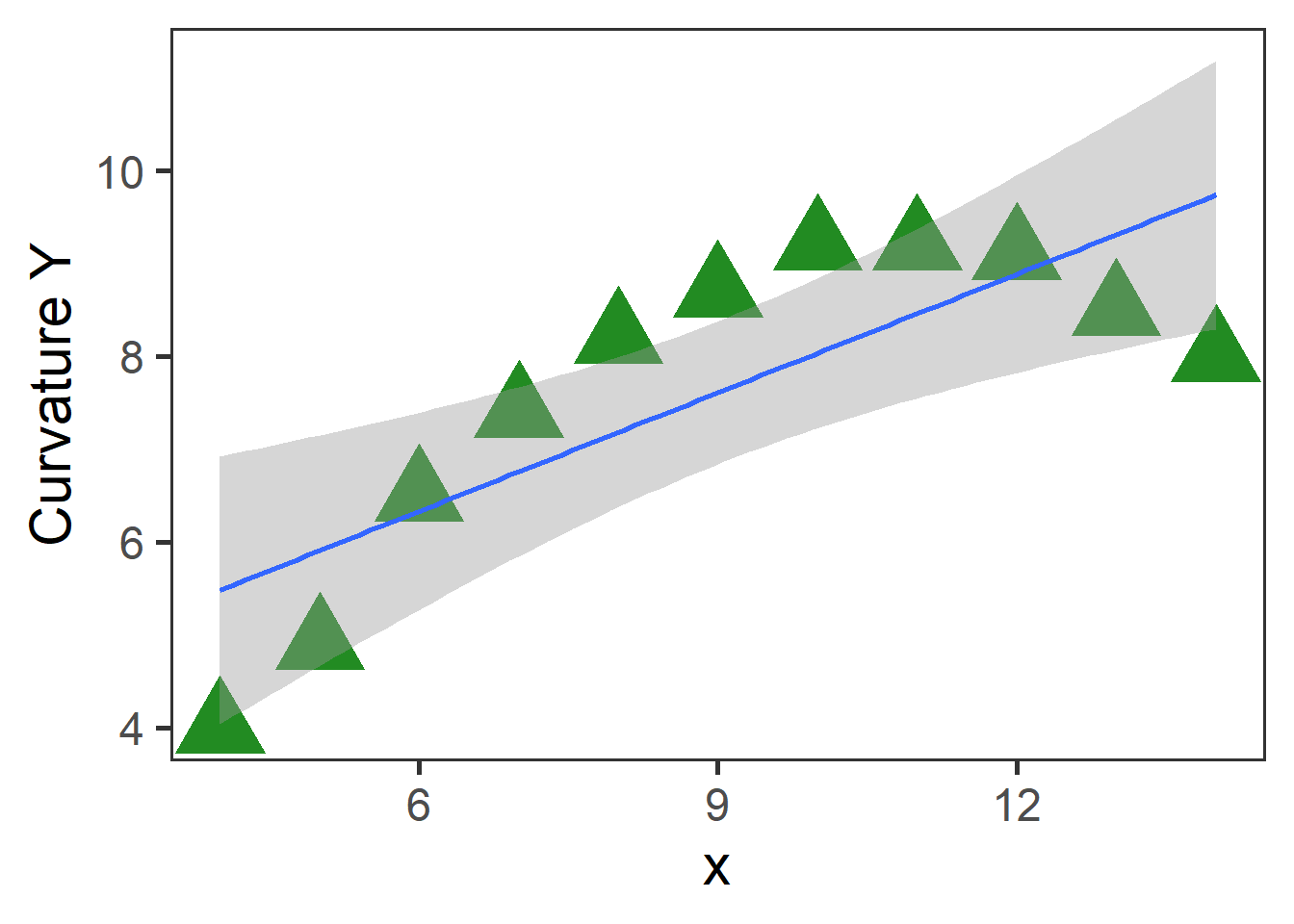
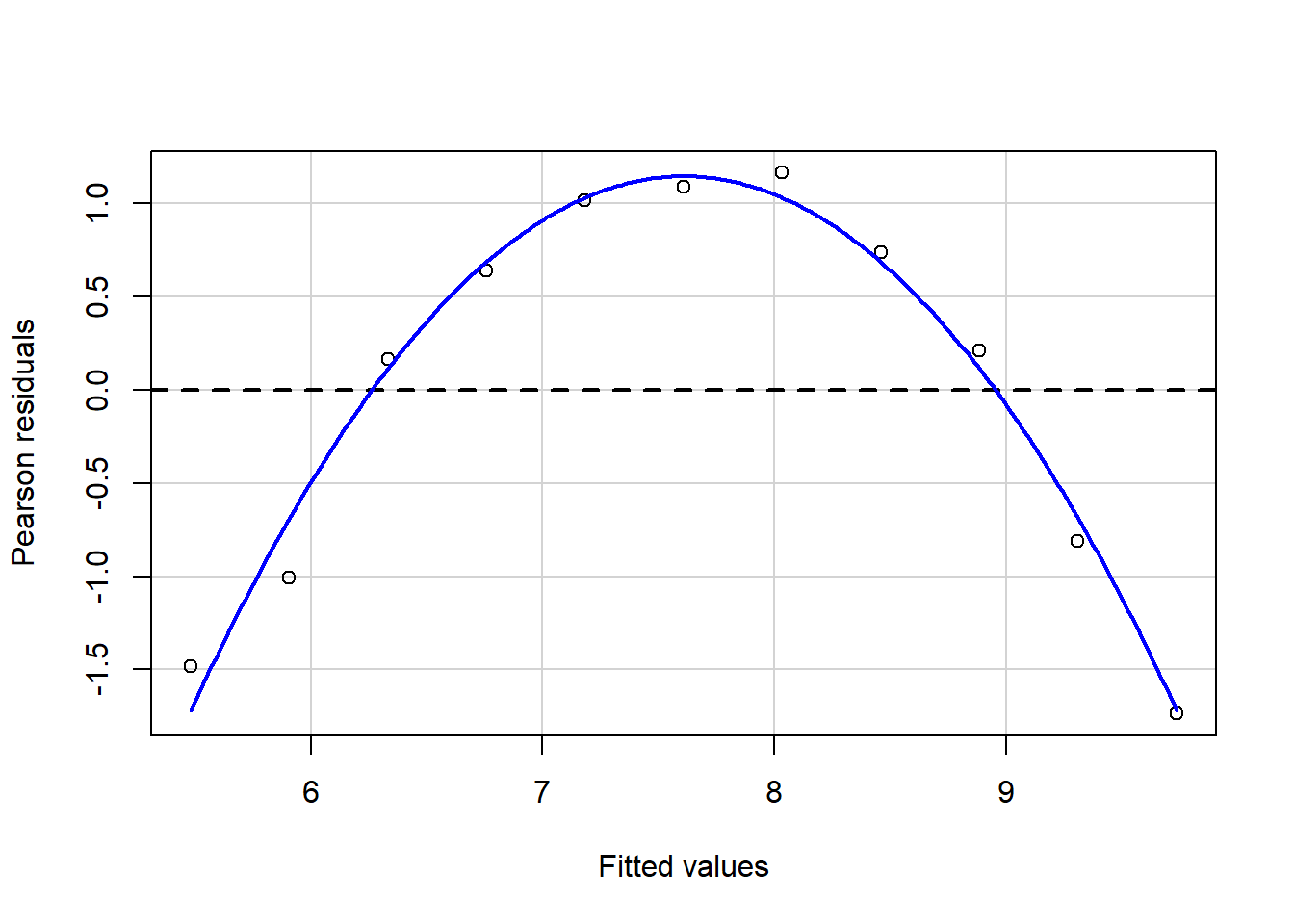
fit.1<-lm(Curvature~x,plots)
residualPlot(fit.1)
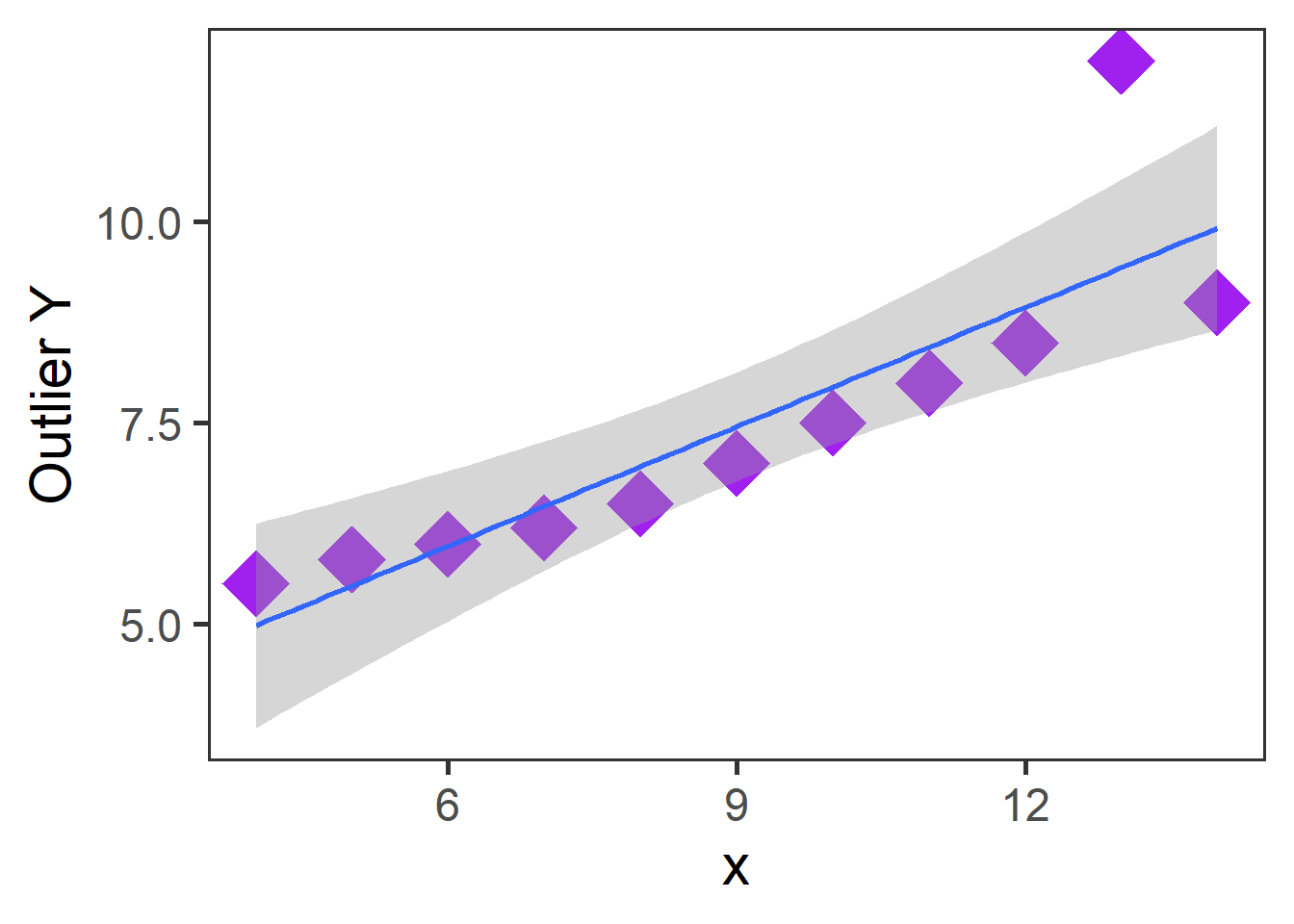
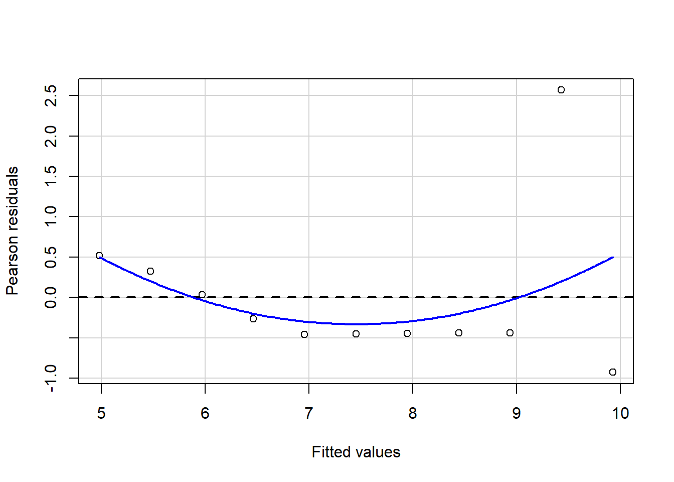
fit.1<-lm(Outlier~x,plots)
residualPlot(fit.1)
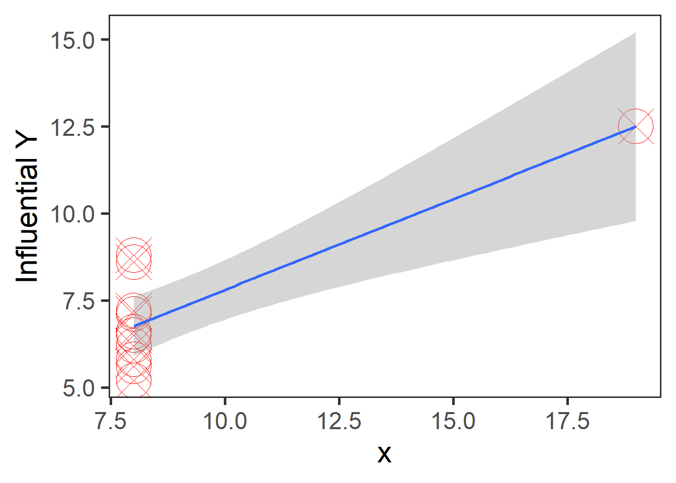
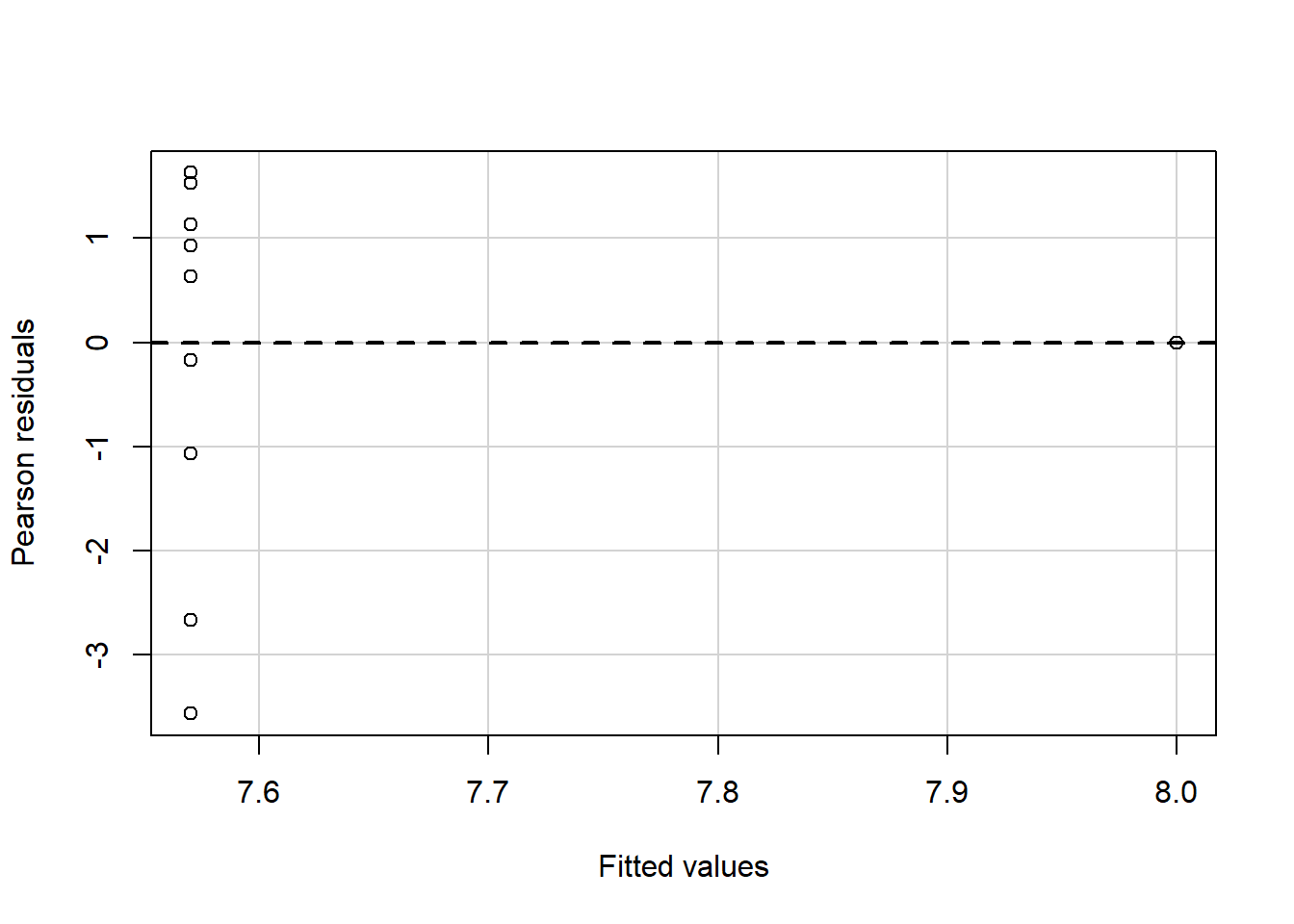
fit.1<-lm(Curvature~c(rep(8,10),19),plots) #data in different formats
residualPlot(fit.1)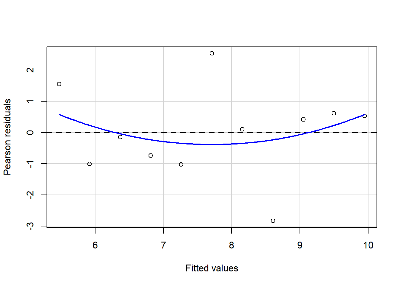
The best residuals sit on the 0 line (y-axis) but in general, the closer to this line, the better. Similarly, they are scattered along with the extent of x. If the residual plot demonstrates either residuals or variance of residuals is not constant, then we must conclude that the model is incorrect in some respect. Still, we may not be able to tell if the problem is due to a misspecified mean function or a misspecified variance function.. Now, let’s use our algae data and fit a regression to analyze some indicators.
fit1<-lm(NO3~mxPH+Cl,data=algae)
#residuals<- fit1$residuals
plot(fit1$residuals)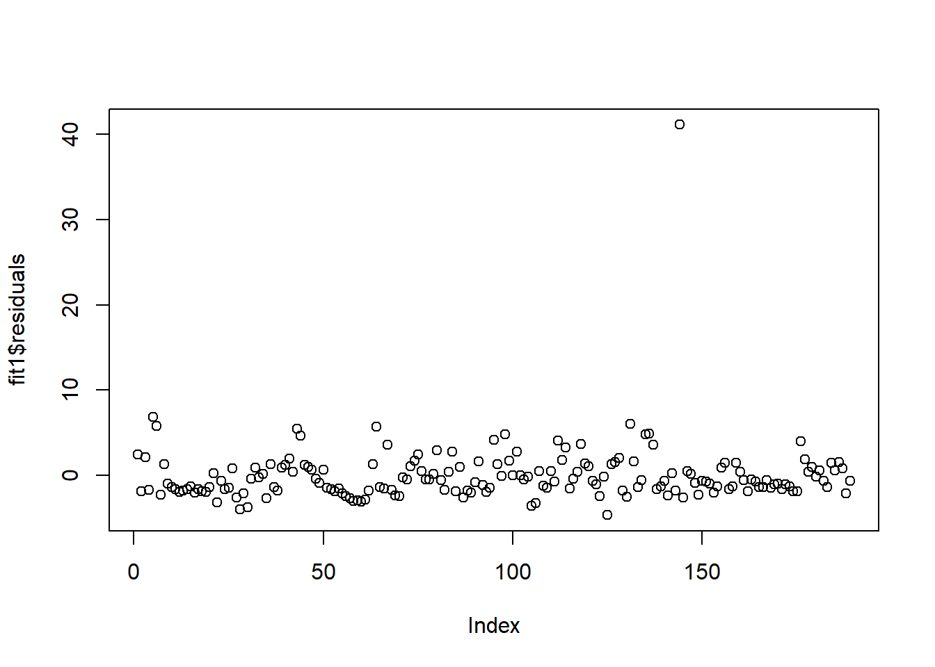
In these datasets, we have one clear outlier, so we should treat that observation. We can also plot residuals against individual predictors \(x_k\).
plot(x = fit1$model$mxPH,y = fit1$residuals)
abline(0,0)
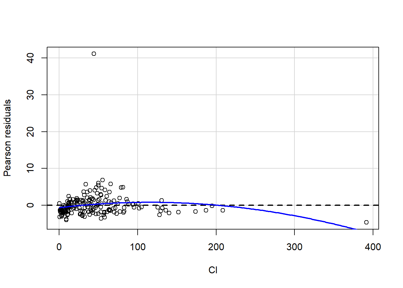
a<-car::residualPlot(fit1,variable="Cl")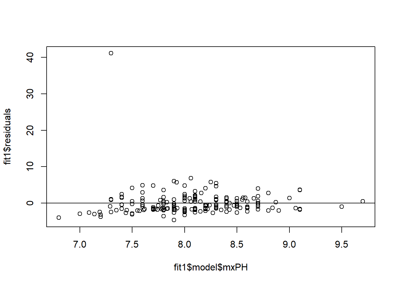
There are a few packages for these tests, and we will have a look at a ggplot2 option.
x<-olsrr::ols_plot_resid_fit(fit1,print_plot = F)+
  theme_bw()
ggplotly(x)
olsrr has many different plots. You can have a look at its package information to build great ordinary least squares regression models.
Testing for Nonconstant Variance
Breusch–Pagan test determines whether the variance of the errors from a regression model depends on the independent variables’ values. In that case, heteroskedasticity is present. If the test statistic has a p-value below an appropriate threshold (e.g., p < 0.05), then the null hypothesis of homoskedasticity is rejected, and heteroskedasticity is assumed.
ncvTest(fit1)
## Non-constant Variance Score Test
## Variance formula: ~ fitted.values
## Chisquare = 62.73071, Df = 1, p = 2.3699e-15
Here, we conclude that there is heteroskedasticity (bad), so the variation of our terms depends on the values of the independent variable. There are a few common ways to fix heteroscedasticity:
- Transform the dependent variable; take the log of the dependent variable.
- Redefine the dependent variable by adding something like a rate.
- Use weighted regression week 6.
- Lastly, we can perform a different model by removing those outliers (Next Week).